Introduction
A few years ago I woke up to an epiphany, realising that I was becoming my dad. I had started a campaign of dealing with wastefulness, switching off lights and eating leftovers to name but a few examples. I set out to transform our menu planning and the weekly food shop as part of this crusade.
Menu planning is a chore which comes easily to some. For others like me, though, it is just another thing to think about on top of an already busy life. Admittedly, it gets easier once establishing a routine, but holidays and the like upsets the momentum and things move back to square one.
Food planning, especially for a young family is essential, without which it can get out of hand and quickly become expensive and wasteful.
I decided that it was not going to beat me! I reached into my bag of tricks and conjured a helper to tackle this quest. A simple piece of R code creates a randomised ‘inspiration’ menu plan. It meant that I had to document a few dozen recipes to start, but the effort soon paid off.
It is now a ton easier to plan our weekly menu plan, and we tend not to use the program anymore. However, it served as a bootstrap, transforming food planning into what is now a routine and straightforward task.
Code
Library
Load the packages used in the demonstration.
package_list <- c("tidyverse", "readxl", "lubridate", "knitr", "kableExtra")
invisible(suppressPackageStartupMessages(lapply(package_list, library, character.only = TRUE)))
rm(package_list)
Functions
The functions below primarily helps with presentation and formatting. The embedded comments describe the working and sequence of each function. I have previously written about these functions and how they are used.
func_rename <-
  function(x) {

    # sequence is important here
    # regex removing all chars not alpha-numeric, underscore or period
    gsub("[^[:alnum:] \\_\\.]", "", x) %>%

      # replace any space or period with underscore
      str_replace_all(pattern = " |\\.", replacement = "\\_") %>%

      # replace multiple underscores with one
      str_replace_all(pattern = "\\_+", replacement = "\\_") %>%

      # remove trailing underscores and period
      str_remove(pattern = "\\_$|\\.$")
  }

func_legible_boolean <-

  # returns `feature name` when TRUE and "Not_" + `feature name` otherwise
  function(df) {

    # add row numbers to input dataframe
    df <-
      df %>%
      ungroup() %>%
      mutate(row_id = row_number())

    # select row_id and other logical fields
    tmp <-
      df %>%
      select(row_id, select_if(., is.logical) %>% names(.)) %>%

      # gather all logical fields and keep row_id to retain identity
      gather(key, value,-row_id) %>%

      # when value is TRUE then return the feature name else "Not_" pasted in
      # front of it
      mutate(value = case_when(
        value ~ key,
        TRUE ~ paste("Not", key, sep = "_")
      )) %>%

      # return the feature names back to header positions
      spread(key, value)

    vars <-
      df %>%
      select_if(is.logical) %>%
      names()

    df %>%

      # return all values from the table after excluding the original logical
      # fields and join the newly adjuted features back into the table using the
      # row_id
      select(-(!!vars)) %>%
      inner_join(tmp,
                 by = "row_id") %>%

      # remove the row_id as the join is complete
      select(-row_id)
  }

func_create_summary <-

  # group by factors, summarising numeric fields to sum total
  function(df) {

    # create a list of factors from the input dataframe
    tmp_factors <- df %>% select_if(is.factor) %>% names()

    # mutate all factors in the dataframe to characters
    df <- df %>% ungroup() %>% mutate_if(is.factor, as.character)


    # list original dataframe with a newly created summary row
    list(

      # original input dataframe
      df,

      # summary row, replaceing each factor value to "Total"
      df %>%
        mutate_at(tmp_factors, ~"Total") %>%

        # group by for each of the original factor features
        group_by_at(tmp_factors) %>%

        # summarise all numeric values to sum total, ignoring NULL values
        summarise_if(is.numeric, sum, na.rm = TRUE)
    ) %>%

      # union all tables contained in the list, including original dataframe and
      # newly created summary row
      reduce(union_all) %>%

      # change factors back into factors
      mutate_at(tmp_factors, factor) %>%
      return()
  }

func_present_headers <-
  function(.) {

    # replace all `spaceholder underscores` with spaces
    str_replace_all(., pattern = "_", replacement = " ") %>%

      # change all words in string to title text
      str_to_title() %>%
      return()
  }

func_change_order <-
  function(df) {

    # please note this function is relatively simple, assuming a split between
    # character and numeric fields only.  the function can easily be amended, or
    # easier still is to coerce the calling dataframe fields to support the use
    # of this function
    df %>%

      # select the calling dataframe character fields first
      select_if(is.character) %>%
      cbind(

        # add numeric fields behind the character fields
        df %>%
          select_if(is.numeric)
      ) %>%
      return()
  }
Parameters and Configuration
The following code block sets configurable parameters, pointing to the source data file location and the decimal accuracy when parsing numbers.
var_path <- "../../resources/family_food_budget/"
options(digits=9)
Import
I’ve previously created a spreadsheet with menu items, underlying ingredients and associated information. Next we import each tab from the Excel file as per the var_path parameter into the df_import dataframe, nesting each tab in the file column.
df_import <-

  # list all files matching the pattern in the parametarised set location
  list.files(path = var_path,
             pattern = "^family.+",
             recursive = TRUE) %>%

  # move the list of files into a tibble, changing the default column name
  # `value` to file_name_ext, representing the file name and extention
  enframe(name=NULL) %>%
  rename(file_name_ext = value) %>%

  # complete the file path used by the read_excel function
  mutate(file_path = paste(var_path, file_name_ext, sep = "/")) %>%

  # read all file tabs for the file and unnest
  mutate_at("file_path", list(file_tab = map), readxl::excel_sheets) %>%
  unnest() %>%

  # import the file using the file_path and file_tab as parameters
  mutate(file = map2(file_path, file_tab, function(file_path, file_tab) {
    readxl::read_excel(path = file_path,
                       sheet = file_tab,
                       guess_max = 100000)
  })) %>%

  # remove redundant variables
  select(-file_path,-file_name_ext)
Let’s inspect the dataframe with the imported data and the delve into a sample of each nested tables too.
df_import## # A tibble: 2 x 2
## file_tab file
## <chr> <list>
## 1 price_list <tibble [46 × 2]>
## 2 menu <tibble [60 × 4]>The dataframe df_import reveals two imported tabs, including price_list and menu.
The price_list data (File Tab = Price List) contains ingredients, units purchased according to the packaging and its purchase price.
Tibble menu (File Tab = Menu) is a list of meals, listing the Meal time-of-day, including breakfast, lunch, dinner or a snack only. Each menu item (meal) contains a list of ingredients and units consumed in the associated menu meal.
The head of each table shown below, corresponding with the File Tab reference described above.
list(
  df_import %>%
    head(1) %>%
    unnest() %>%
    select(-file_tab) %>%
    rename_all(func_present_headers) %>%
    mutate_at("Price", ~ scales::dollar(., prefix = "£")) %>%
    head(),
  df_import %>%
    tail(1) %>%
    unnest() %>%
    select(-file_tab) %>%
    rename_all(func_present_headers) %>%
    head()
) %>%
  reduce(dplyr::bind_cols) %>%
  kable(
    format = "html",
    col.names = c(
      "Item",
      "Price",
      "Meal",
      "Menu",
      "Item",
      "Unit"
    )
  ) %>%
  kableExtra::kable_styling(full_width = TRUE, font_size = 12) %>%
  kableExtra::collapse_rows(columns = 3:4,  valign = "top") %>%
  add_header_above(
    c("Price List" = 2, "Menu" = 4),
    align = "c",
    color = "white",
    bold = TRUE,
    background = "grey"
)| Item | Price | Meal | Menu | Item | Unit |
|---|---|---|---|---|---|
| Baby Carrots | £1.30 | Dinner | Fish fingers, Mash & Beans | Fish | 0.50 |
| Bacon | £2.00 | Potatoes | 0.25 | ||
| Baked Beans | £2.50 | Baked Beans | 0.25 | ||
| Bread | £1.00 | Sausage, Mash & Beans | Sausage | 1.00 | |
| Broccoli | £1.30 | Potatoes | 0.25 | ||
| Burger Buns | £1.00 | Baked Beans | 0.25 |
Reference Period
Here we instantiate two reference tibbles, including the period or timeframe for which the meals are planned, and the meal time-of-day.
Tibble ref_days_join_meal is a cartesian product of ref_days, expanding meal times for each day, as listed in the ref_meal_time tibble.
ref_days <-
  seq.Date(from = ymd("2019-06-01"),
           to = ymd("2019-06-30"),
           by = "day") %>%
  enframe(name=NULL) %>%
  rename(Day = value)

ref_meal_time <-
  c("Breakfast", "Snack", "Lunch", "Dinner") %>%
  factor(ordered = TRUE) %>%
  enframe(name=NULL) %>%
  rename(Meal = value)

ref_days_join_meal <-
  ref_days %>%

  # expand each day with the 4 mealtimes, creating a dataframe with combinations
  # of all days and mealtimes.
  expand(Day, Meal = ref_meal_time$Meal) %>%

  # extract some attributes from the days, including the weekday, and the first
  # day of the week `SOW`
  mutate(Weekday = wday(Day,  label = TRUE)) %>%
  mutate(SOW = floor_date(Day, week_start = 1, unit = "week")) %>%
  mutate_at("Weekday",
~fct_relevel(., "Mon", "Tue", "Wed", "Thu", "Fri", "Sat", "Sun"))Function
The function func_random_meal randomises meals for each mealtime, the size matching the number of days by week (SOW) in the ref_days tibble.
The function draws randomly from meals for each mealtime. For example, dinners will only sample from meals classified as dinner.
It avoids sampling with replacement from the available menu meals unless there are fewer meals than the calling days.
func_random_meal <-
  function(param_meal, param_days) {
    # create a parameter with the number of days in the param_days parameter
    param_sample_size <- count(param_days) %>% as.integer()

    # create a parameter, returning the count of items in the meal
    param_menu_item_size <-
      df_menu_items %>%

      # filter by the calling param_meal
      filter(Meal == param_meal) %>%
      nrow()

    # function that returns TRUE if the param_menu_item_size <
    # param_sample_size, enabling the `tmp_meals` function to sample with
    # replacement
    param_replace <-
    if (param_menu_item_size < param_sample_size) {
      TRUE %>% return()
    } else {
      FALSE %>% return()
    }

    # Sample ----
    tmp_meals <-
      df_menu_items %>%

      # filter by the calling param_meal
      filter(Meal == param_meal) %>%

      # create a sample size according the the parameter param_sample_size,
      # enabling replacement if the param_menu_item_size < param_sample_size
      sample_n(size = param_sample_size, replace = param_replace) %>%
      ungroup() %>%

      # remove unecessary attributes
      select(-Meal,-Meal_item) %>%

      # add row number
      mutate(Day_order = row_number())

    # Join ----
    param_days %>%

      # join the newly created tibble `tmp_meals` to the param_days tibble,
      # using the Day_order as key to join
      mutate(Day_order = row_number()) %>%
      inner_join(tmp_meals, by = "Day_order") %>%
      return()
  }
Randomise Meals
We start of by setting a seed, thus making results repeatable.
Next, we create a new tibble df_meal_plan by passing the meals for each week to the func_random_meal function, generating and returning a random list of meals to the Menu column.
Menu_Cost summarises the total cost of all underlying ingredients for the meal.
Executing the code block outputs the head of the new tibble for inspection.
set.seed(567)
# set seed to make the results repeatable

df_meal_plan <-
  # for each day and mealtime combination
  ref_days_join_meal %>%

  # group by week and mealtime, and nest all days within it
  group_by(SOW, Meal) %>%
  nest(Weekday, Day) %>%

  # map the meal and nested days to the `func_random_meal` function and return
  # result to the Menu column
  mutate(Menu  = map2(Meal, data, func_random_meal)) %>%

  # unnest the result and arrange the output
  unnest(Menu) %>%
  arrange(SOW, Weekday, Meal) %>%
  mutate_at("SOW", ~ paste0(format(., "%yW%W: "),
                           format(., "%d %b - "),
                           format(. + 6, "%d %b")) %>%
              factor(., ordered = TRUE))

# check the results by printing the first day worth of meals
df_meal_plan %>%
  head(4) %>%

  # change the date formatting for improved presentation
  mutate_if(is.Date, format, format = "%d-%b") %>%

  # presentation options
  mutate_at("Menu_Cost", ~scales::dollar(., prefix = "£")) %>%
  rename_all(func_present_headers) %>%
  kable(format = "html") %>%
kableExtra::kable_styling(full_width = FALSE, font_size = 10)| Sow | Meal | Weekday | Day | Day Order | Menu | Menu Cost | Ingredients |
|---|---|---|---|---|---|---|---|
| 19W21: 27 May - 02 Jun | Breakfast | Sat | 01-Jun | 1 | Rice Pops | £0.25 | list(file_tab = “menu”, Item = “Rice Pops”, Unit = 0.25, Price = 1, Cost = 0.25) |
| 19W21: 27 May - 02 Jun | Dinner | Sat | 01-Jun | 1 | Carbonara | £3.36 | list(file_tab = c(“menu”, “menu”, “menu”, “menu”, “menu”), Item = c(“Bacon”, “Mushrooms”, “Cheese”, “Onion”, “Pasta”), Unit = c(0.66, 0.35, 0.33, 0.15, 0.05), Price = c(2, 1, 4, 1.5, 3), Cost = c(1.32, 0.35, 1.32, 0.225, 0.15)) |
| 19W21: 27 May - 02 Jun | Lunch | Sat | 01-Jun | 1 | Sandwich Ham & Cheese | £1.85 | list(file_tab = c(“menu”, “menu”, “menu”), Item = c(“Bread”, “Ham”, “Cheese”), Unit = c(0.35, 0.35, 0.2), Price = c(1, 2, 4), Cost = c(0.35, 0.7, 0.8)) |
| 19W21: 27 May - 02 Jun | Snack | Sat | 01-Jun | 1 | Fruit | £0.62 | list(file_tab = “menu”, Item = “Fruit”, Unit = 0.125, Price = 5, Cost = 0.625) |
Month Lookahead
This section is really what this whole exercise is about!
We’ve created random meals for a period, ready to print a copy of the first output and pin it to the family whiteboard. We now have a menu plan for the month ahead - result.
The second output is used for budgeting the food bill once we have taken stock, and calculate what is to be purchased to satisfy the newly created budget plan.
# Meal ----
df_meal_plan %>%
  select(SOW, Weekday, Meal, Menu) %>%
  spread(Weekday, Menu, fill = "--") %>%
  ungroup() %>%
  mutate_at("SOW", format, format = "%yW%W") %>%
  mutate_at("Meal", factor, levels = ref_meal_time$Meal) %>%
  arrange(SOW, Meal) %>%
  kable(format = "html", align = "c") %>%
  kable_styling("striped", full_width = FALSE, font_size = 10) %>%
  column_spec(1, bold = TRUE) %>%
collapse_rows(columns = 1:2, valign = "top")| SOW | Meal | Mon | Tue | Wed | Thu | Fri | Sat | Sun |
|---|---|---|---|---|---|---|---|---|
| 19W21: 27 May - 02 Jun | Breakfast | – | – | – | – | – | Rice Pops | Honey Hoops |
| Snack | – | – | – | – | – | Fruit | Fruit | |
| Lunch | – | – | – | – | – | Sandwich Ham & Cheese | Sandwich Tuna | |
| Dinner | – | – | – | – | – | Carbonara | Baked Potato & Humous | |
| 19W22: 03 Jun - 09 Jun | Breakfast | Honey Hoops | Honey Hoops | Honey Hoops | Weetabix | Honey Hoops | Honey Hoops | Weetabix |
| Snack | Fruit | Fruit | Fruit | Fruit | Fruit | Fruit | Fruit | |
| Lunch | Sandwich Ham & Cheese | Sandwich Gammon | Sandwich Ham & Cheese | Sandwich Tuna | Sandwich Tuna | Sandwich Tuna | Sandwich Gammon | |
| Dinner | Fish fingers, Mash & Beans | Rice Dish Chicken | Carbonara | Roast Dinner | Spag Bol | Rice Dish Gammon | Daddy’s Chicken & Curry | |
| 19W23: 10 Jun - 16 Jun | Breakfast | Rice Pops | Rice Pops | Weetabix | Weetabix | Weetabix | Rice Pops | Weetabix |
| Snack | Fruit | Fruit | Fruit | Fruit | Fruit | Fruit | Fruit | |
| Lunch | Sandwich Tuna | Sandwich Gammon | Sandwich Gammon | Sandwich Tuna | Sandwich Tuna | Sandwich Gammon | Sandwich Tuna | |
| Dinner | Baked Potato & Humous | Rice Dish Gammon | Spag Bol | Daddy’s Chicken & Curry | Fish fingers, Mash & Beans | Roast Dinner | Carbonara | |
| 19W24: 17 Jun - 23 Jun | Breakfast | Honey Hoops | Weetabix | Rice Pops | Honey Hoops | Honey Hoops | Honey Hoops | Weetabix |
| Snack | Fruit | Fruit | Fruit | Fruit | Fruit | Fruit | Fruit | |
| Lunch | Sandwich Tuna | Sandwich Tuna | Sandwich Tuna | Sandwich Gammon | Sandwich Tuna | Sandwich Gammon | Sandwich Gammon | |
| Dinner | Fish fingers, Mash & Beans | Burgers & Hotdogs | Rice Dish Gammon | Rice Dish Chicken | Daddy’s Chicken & Curry | Roast Dinner | Sausage, Mash & Beans | |
| 19W25: 24 Jun - 30 Jun | Breakfast | Honey Hoops | Rice Pops | Weetabix | Weetabix | Honey Hoops | Weetabix | Weetabix |
| Snack | Fruit | Fruit | Fruit | Fruit | Fruit | Fruit | Fruit | |
| Lunch | Sandwich Gammon | Sandwich Tuna | Sandwich Tuna | Sandwich Ham & Cheese | Sandwich Ham & Cheese | Sandwich Gammon | Sandwich Ham & Cheese | |
| Dinner | Carbonara | Burgers & Hotdogs | Rice Dish Chicken | Baked Potato & Humous | Roast Dinner | Fish fingers, Mash & Beans | Sausage, Mash & Beans |
# Money ----
df_meal_plan %>%
  group_by(SOW, Weekday, Meal) %>%
  summarise_at("Menu_Cost", sum, na.rm = TRUE) %>%
  spread(Weekday, Menu_Cost) %>%
  ungroup() %>%
  mutate_at("SOW", format, format = "%yW%W") %>%
  mutate_at("Meal", factor, levels = ref_meal_time$Meal) %>%
  arrange(SOW, Meal) %>%
  func_create_summary() %>%
  mutate_at(c("SOW", "Meal"), as.character) %>%
  group_by_if(is.character) %>%
  nest(.key = "Total") %>%
  mutate(data = Total) %>%
  mutate_at("Total", map, rowSums, na.rm = TRUE) %>%
  unnest() %>%
  mutate_if(is.numeric, ~scales::dollar(., prefix = "£")) %>%
  mutate_if(is.character, str_replace, pattern = "£NA", replacement = "--") %>%
  kable(format = "html", align = "c") %>%
  kable_styling("striped", full_width = FALSE, font_size = 10) %>%
  column_spec(1, bold = TRUE) %>%
collapse_rows(columns = 1:2, valign = "top")| SOW | Meal | Total | Mon | Tue | Wed | Thu | Fri | Sat | Sun |
|---|---|---|---|---|---|---|---|---|---|
| 19W21: 27 May - 02 Jun | Breakfast | £0.50 | – | – | – | – | – | £0.25 | £0.25 |
| Snack | £1.25 | – | – | – | – | – | £0.62 | £0.62 | |
| Lunch | £4.70 | – | – | – | – | – | £1.85 | £2.85 | |
| Dinner | £5.52 | – | – | – | – | – | £3.36 | £2.15 | |
| 19W22: 03 Jun - 09 Jun | Breakfast | £1.90 | £0.25 | £0.25 | £0.25 | £0.32 | £0.25 | £0.25 | £0.32 |
| Snack | £4.38 | £0.62 | £0.62 | £0.62 | £0.62 | £0.62 | £0.62 | £0.62 | |
| Lunch | £14.45 | £1.85 | £1.10 | £1.85 | £2.85 | £2.85 | £2.85 | £1.10 | |
| Dinner | £27.70 | £2.88 | £3.24 | £3.36 | £6.32 | £3.16 | £1.97 | £6.77 | |
| 19W23: 10 Jun - 16 Jun | Breakfast | £2.05 | £0.25 | £0.25 | £0.32 | £0.32 | £0.32 | £0.25 | £0.32 |
| Snack | £4.38 | £0.62 | £0.62 | £0.62 | £0.62 | £0.62 | £0.62 | £0.62 | |
| Lunch | £14.70 | £2.85 | £1.10 | £1.10 | £2.85 | £2.85 | £1.10 | £2.85 | |
| Dinner | £26.61 | £2.15 | £1.97 | £3.16 | £6.77 | £2.88 | £6.32 | £3.36 | |
| 19W24: 17 Jun - 23 Jun | Breakfast | £1.90 | £0.25 | £0.32 | £0.25 | £0.25 | £0.25 | £0.25 | £0.32 |
| Snack | £4.38 | £0.62 | £0.62 | £0.62 | £0.62 | £0.62 | £0.62 | £0.62 | |
| Lunch | £14.70 | £2.85 | £2.85 | £2.85 | £1.10 | £2.85 | £1.10 | £1.10 | |
| Dinner | £29.55 | £2.88 | £5.00 | £1.97 | £3.24 | £6.77 | £6.32 | £3.38 | |
| 19W25: 24 Jun - 30 Jun | Breakfast | £2.05 | £0.25 | £0.25 | £0.32 | £0.32 | £0.25 | £0.32 | £0.32 |
| Snack | £4.38 | £0.62 | £0.62 | £0.62 | £0.62 | £0.62 | £0.62 | £0.62 | |
| Lunch | £13.45 | £1.10 | £2.85 | £2.85 | £1.85 | £1.85 | £1.10 | £1.85 | |
| Dinner | £26.33 | £3.36 | £5.00 | £3.24 | £2.15 | £6.32 | £2.88 | £3.38 | |
| NA | Total | £204.86 | £23.42 | £26.68 | £24.04 | £30.86 | £33.11 | £33.30 | £33.46 |
Purchasing
The following section is creating output that helps to manage the newly created menu plan.
The newly created menu plans now enables one to project spend and even create a shopping list for each week1.
df_meal_plan_purchases <-
  df_meal_plan %>%
  unnest() %>%
  select(Day, Item, Unit, Price, Cost) %>%
  mutate(Meals = 1) %>%
  group_by(Item) %>%
  mutate_at(c("Unit", "Meals"), list(cum = cumsum)) %>%
  mutate_at("Unit_cum", ceiling) %>%
  mutate_at("Unit_cum", list(buy = ~. != lead(.),
                             buy_volume = ~lead(.) - .)) %>%
  mutate(Cost_cum = Unit_cum * Price) %>%
  mutate_at("Day",
            list(SOW = floor_date),
            unit = "week",
            week_start = 1) %>%
  group_by(SOW, add = TRUE) %>%
  summarise_at("buy_volume", sum, na.rm = TRUE)

df_plot <-
  df_meal_plan_purchases %>%
  inner_join(
    df_import %>%
      filter(file_tab == "price_list") %>%
      unnest(),
    by = "Item"
  ) %>%
  filter(buy_volume > 0) %>%
  mutate(Cost = Price * buy_volume) %>%
  ungroup() %>%
  mutate(Total_Cost = sum(Cost, na.rm = TRUE)) %>%
  arrange(desc(Total_Cost)) %>%
  mutate_at("Item", fct_inorder) %>%
  group_by(SOW, add = FALSE) %>%
  mutate_at("Cost", list(Cost_Cum = cumsum)) %>%
  ungroup() %>%
  arrange(SOW) %>%
  mutate_at("SOW", ~ paste0(format(., "%yW%W: "),
                           format(., "%d %b - "),
                           format(. + 6, "%d %b")) %>%
              factor(., ordered = TRUE))

df_plot %>%
  ggplot(aes(x = Item, y = Cost, fill = Cost)) +
  geom_col() +
  geom_line(aes(y = Cost_Cum, group = SOW)) +
  ggrepel::geom_label_repel(
    data = df_plot %>%
      group_by(SOW, add = FALSE) %>%
      top_n(n = 1, wt = Cost_Cum),
    aes(y = Cost_Cum, label = scales::dollar(Cost_Cum, prefix = "£")),
    fill = "white"
  ) +
  facet_grid(SOW ~ ., switch = "y") +
  scale_y_continuous(labels = scales::dollar_format(prefix = "£")) +
  scale_fill_continuous(labels = scales::dollar_format(prefix = "£")) +
  theme_classic() +
  theme(
    axis.text.x = element_text(angle = 90, hjust = 1),
    strip.placement = "outside",
    strip.text.y = element_text(angle = 180, vjust = 1),
    strip.background.y = element_blank(),
    legend.position = "bottom",
    legend.key.width=unit(2.5,"cm")
  ) +
  labs(title = "Monthly shopping costs by week",
       y = "Purchases")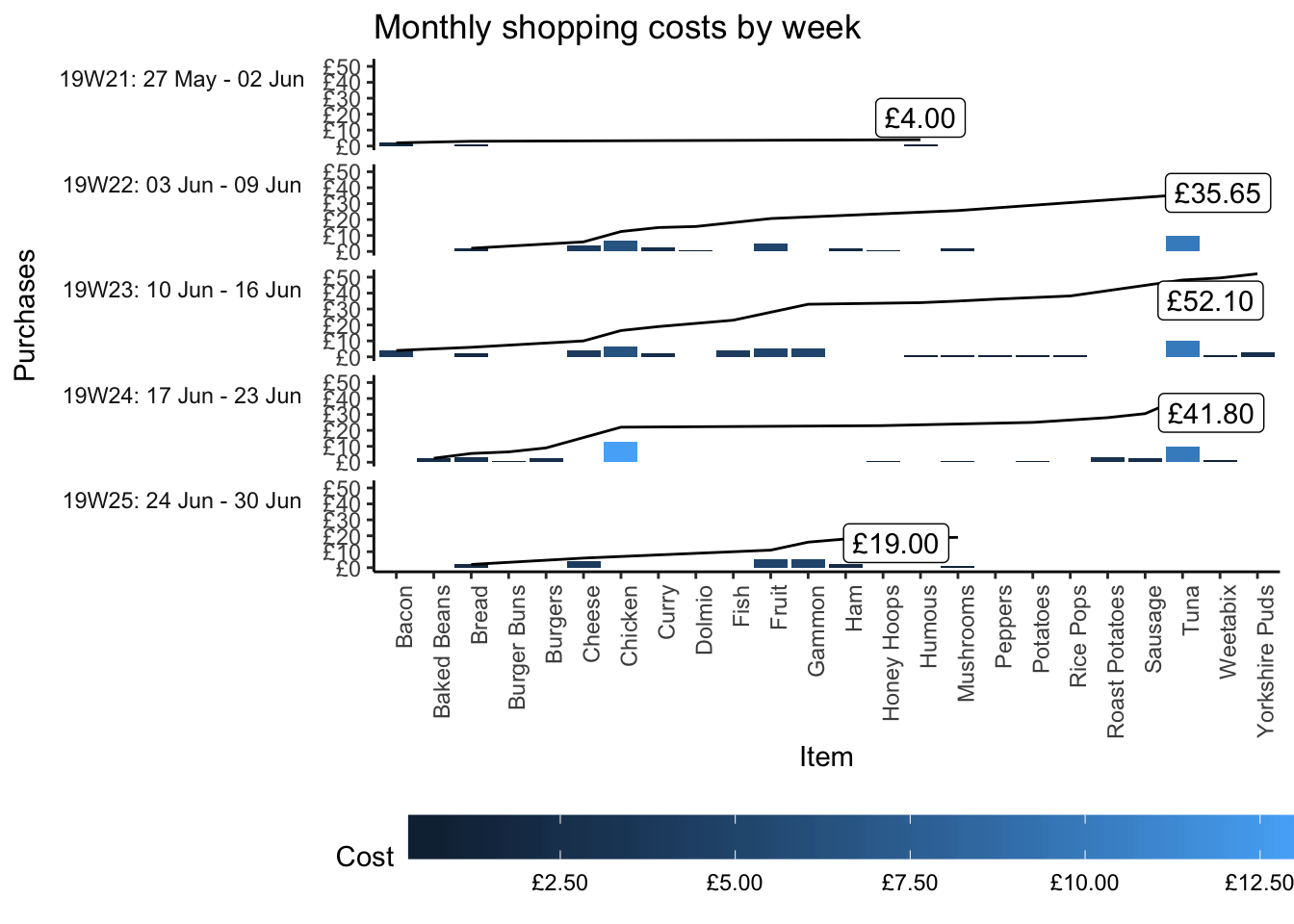
The Shopping List
Being able to estimate my food bill is a result. However, having a prospective shopping list is practical and useful.
func_output_group_item_table <-
  function(param_group, param_group_selector) {
    # print the distinct grouping category as header
    cat(paste0(
      "<h4>",
      str_replace_all(param_group, pattern = "_", replacement = " "),
      "</h4>"
    ))

    df_plot <-
      df_plot %>%
      select(SOW, Item, volume = buy_volume, Price, Cost, Cost_Cum)

    df_plot %>%
      # filter the master data by the grouping category parameter
      filter(!!param_group_selector == param_group) %>%
      ungroup() %>%

      #  remove the grouping category from it
      select(-!!param_group_selector) %>%

      # create a row with a sum total for each numeric column
      mutate_at("Cost_Cum", as.character) %>%
      func_create_summary() %>%

      # styling and presentation options executed next, as described in the
      # previous code block
      mutate_at("volume", as.character) %>%
      mutate_at("Cost_Cum", as.numeric) %>%
      rename_all(func_present_headers) %>%
      mutate_if(is.numeric, ~ round(., 2) %>% scales::dollar(., prefix = "£")) %>%
      mutate_if(is.character, str_remove, pattern = "\\£NA") %>%
      mutate_if(is.factor,
                str_replace_all,
                pattern = "_",
                replacement = " ") %>%
      kable(align = "r", format = "html") %>%
      kableExtra::kable_styling(full_width = FALSE,
                                font_size = 12) %>%
      kableExtra::collapse_rows(columns = 1:4, valign = "middle") %>%
      return()
  }

func_output_group_item_table_iterator <-
  function(param_group_selector) {
    for (param_group in (df_plot %>%
                         distinct(!!param_group_selector) %>%
                         pull()))  {
      func_output_group_item_table(param_group, param_group_selector) %>% print()
    }
  }

func_output_group_item_table_iterator(quo(SOW))
19W21: 27 May - 02 Jun
| Item | Volume | Price | Cost | Cost Cum |
|---|---|---|---|---|
| Bacon | 1 | £2 | £2 | £2 |
| Bread | £1 | £1 | £3 | |
| Humous | £4 | |||
| Total | 3 | £4 | £4 |
19W22: 03 Jun - 09 Jun
| Item | Volume | Price | Cost | Cost Cum |
|---|---|---|---|---|
| Bread | 2 | £1.00 | £2.00 | £2.00 |
| Cheese | 1 | £4.00 | £4.00 | £6.00 |
| Chicken | £6.50 | £6.50 | £12.50 | |
| Curry | £2.50 | £2.50 | £15.00 | |
| Dolmio | £0.65 | £0.65 | £15.65 | |
| Fruit | £5.00 | £5.00 | £20.65 | |
| Ham | £2.00 | £2.00 | £22.65 | |
| Honey Hoops | £1.00 | £1.00 | £23.65 | |
| Mushrooms | 2 | £2.00 | £25.65 | |
| Tuna | £5.00 | £10.00 | £35.65 | |
| Total | 13 | £28.65 | £35.65 |
19W23: 10 Jun - 16 Jun
| Item | Volume | Price | Cost | Cost Cum |
|---|---|---|---|---|
| Bacon | 2 | £2.00 | £4.00 | £4.00 |
| Bread | £1.00 | £2.00 | £6.00 | |
| Cheese | 1 | £4.00 | £4.00 | £10.00 |
| Chicken | £6.50 | £6.50 | £16.50 | |
| Curry | £2.50 | £2.50 | £19.00 | |
| Fish | £4.00 | £4.00 | £23.00 | |
| Fruit | £5.00 | £5.00 | £28.00 | |
| Gammon | £33.00 | |||
| Humous | £1.00 | £1.00 | £34.00 | |
| Mushrooms | £35.00 | |||
| Peppers | £1.20 | £1.20 | £36.20 | |
| Potatoes | £1.00 | £1.00 | £37.20 | |
| Rice Pops | £38.20 | |||
| Tuna | 2 | £5.00 | £10.00 | £48.20 |
| Weetabix | 1 | £1.30 | £1.30 | £49.50 |
| Yorkshire Puds | £2.60 | £2.60 | £52.10 | |
| Total | 19 | £44.10 | £52.10 |
19W24: 17 Jun - 23 Jun
| Item | Volume | Price | Cost | Cost Cum |
|---|---|---|---|---|
| Baked Beans | 1 | £2.50 | £2.50 | £2.50 |
| Bread | 3 | £1.00 | £3.00 | £5.50 |
| Burger Buns | 1 | £1.00 | £6.50 | |
| Burgers | £2.50 | £2.50 | £9.00 | |
| Chicken | 2 | £6.50 | £13.00 | £22.00 |
| Honey Hoops | 1 | £1.00 | £1.00 | £23.00 |
| Mushrooms | £24.00 | |||
| Potatoes | £25.00 | |||
| Roast Potatoes | £3.00 | £3.00 | £28.00 | |
| Sausage | £2.50 | £2.50 | £30.50 | |
| Tuna | 2 | £5.00 | £10.00 | £40.50 |
| Weetabix | 1 | £1.30 | £1.30 | £41.80 |
| Total | 16 | £28.30 | £41.80 |
19W25: 24 Jun - 30 Jun
| Item | Volume | Price | Cost | Cost Cum |
|---|---|---|---|---|
| Bread | 2 | £1 | £2 | £2 |
| Cheese | 1 | £4 | £4 | £6 |
| Fruit | £5 | £5 | £11 | |
| Gammon | £16 | |||
| Ham | £2 | £2 | £18 | |
| Mushrooms | £1 | £1 | £19 | |
| Total | 7 | £18 | £19 |
EDA
This section explores our menu by mealtime, visualising the ranked cost of menus.
df_meal_plan %>%
  distinct(Meal, Menu, Menu_Cost) %>%
  arrange(Meal, desc(Menu_Cost)) %>%
  mutate_at("Menu", fct_inorder) %>%
  ggplot(aes(x = Menu, y = Menu_Cost, fill = Menu_Cost)) +
  geom_col() +
  geom_label(aes(label = format(Menu_Cost, digits = 2, big.mark = ",", format = "#.##") %>%
                   paste0("£", .)),
             col = "white",
             size = 3) +
  coord_flip() +
  theme_classic() +
  scale_y_continuous(labels = scales::dollar_format(prefix = "£")) +
  facet_grid(Meal ~ .,
             scales = "free_y",
             space = "free",
             switch = "y") +
  theme(strip.placement = "outside",
        strip.text.y = element_text(angle = 180,
                                    face = "bold",
                                    size = 10,
                                    hjust = 0,
                                    vjust = 1),
        strip.background.y = element_blank(),
        plot.subtitle = element_text(size = 8, face = "italic"),
        legend.key.height=unit(0.5,"line"),
        legend.title = element_text(size = 10),
        legend.text = element_text(size = 8),
        legend.position = "bottom") +
  labs(title = "Cost of meals",
       subtitle = "Grouped by mealtime - Ordered by Cost",
       fill = "Cost/ Meal",
       y = "Cost/ Meal",
       x = "")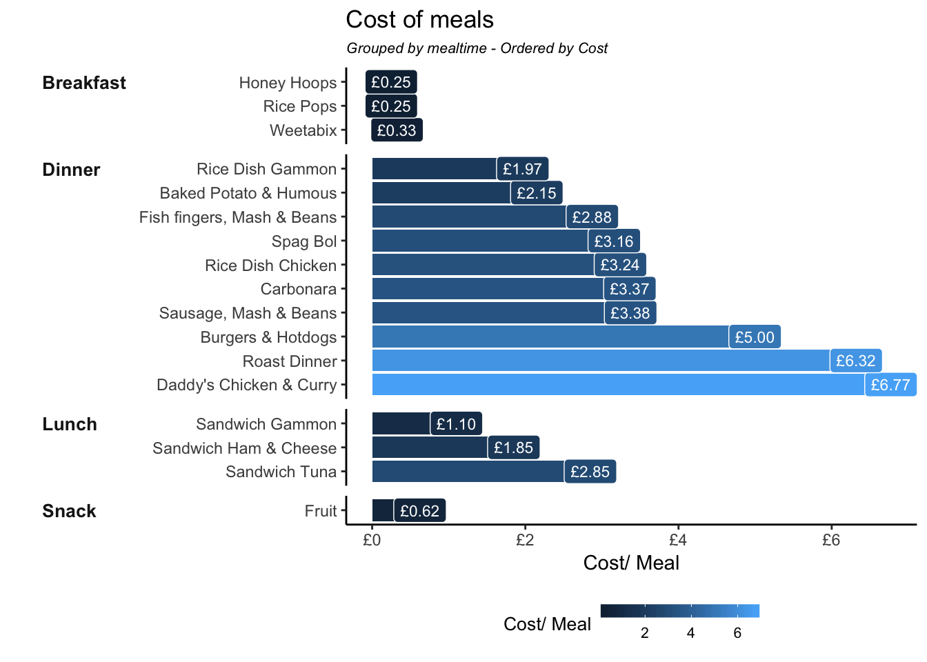
The following visualisation contrasts a few meals to provide a side-by-side breakdown of costs per menu. It is clear that using meat and complexity is what increases the cost of meals.
# Expensive Items ----
df_menu_items %>%
  filter(grepl("curry|roast|spag|carb", Menu, ignore.case = TRUE)) %>%
  unnest() %>%
  arrange(desc(Cost)) %>%
  mutate_at("Item", fct_inorder) %>%
  ggplot(aes(Menu, Cost, fill = Item)) +
  geom_col(position = "stack", show.legend = FALSE) +
  geom_label(
    aes(
      label = format(
        Cost,
        digits = 2,
        big.mark = ",",
        format = "#.##"
      ) %>% paste0("£", .) %>% paste(Item, .)
    ),
    position = "stack",
    col = "white",
    size = 3,
    show.legend = FALSE
  ) +
  scale_y_continuous(labels = scales::dollar_format(prefix = "£")) +
  theme_classic() +
  labs(title = "Comparing the cost of ingredients for selected meals")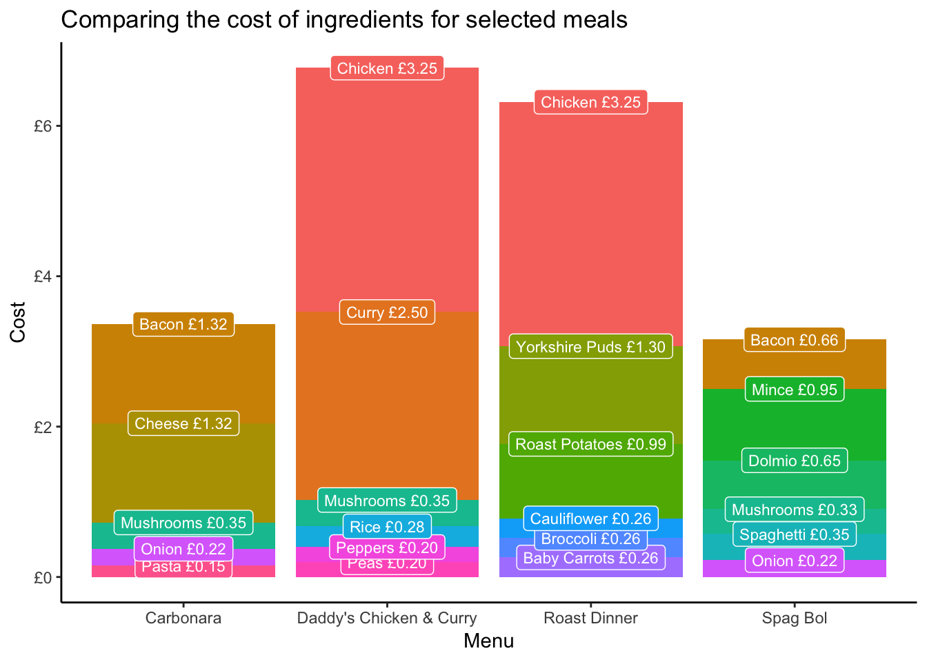
Summary
This post doesn’t describe life-changing methods or insights. However, it demonstrates that coding can be used to solve simple, everyday problems, even having a meaningful impact on my little family. Imagine though what it can do for seemingly insignificant problems in business.
Session
sessionInfo()## R version 3.5.3 (2019-03-11)
## Platform: x86_64-apple-darwin15.6.0 (64-bit)
## Running under: macOS Mojave 10.14.4
##
## Matrix products: default
## BLAS: /Library/Frameworks/R.framework/Versions/3.5/Resources/lib/libRblas.0.dylib
## LAPACK: /Library/Frameworks/R.framework/Versions/3.5/Resources/lib/libRlapack.dylib
##
## locale:
## [1] en_GB.UTF-8/en_GB.UTF-8/en_GB.UTF-8/C/en_GB.UTF-8/en_GB.UTF-8
##
## attached base packages:
## [1] stats graphics grDevices utils datasets methods base
##
## other attached packages:
## [1] kableExtra_1.1.0 knitr_1.22 lubridate_1.7.4 readxl_1.3.1
## [5] forcats_0.4.0 stringr_1.4.0 dplyr_0.8.0.1 purrr_0.3.2
## [9] readr_1.3.1 tidyr_0.8.3 tibble_2.1.1 ggplot2_3.1.1
## [13] tidyverse_1.2.1
##
## loaded via a namespace (and not attached):
## [1] tidyselect_0.2.5 xfun_0.6 reshape2_1.4.3
## [4] haven_2.1.0 lattice_0.20-38 colorspace_1.4-1
## [7] generics_0.0.2 htmltools_0.3.6 viridisLite_0.3.0
## [10] yaml_2.2.0 utf8_1.1.4 rlang_0.3.4
## [13] pillar_1.3.1 glue_1.3.1 withr_2.1.2.9000
## [16] selectr_0.4-1 modelr_0.1.4 plyr_1.8.4
## [19] munsell_0.5.0 blogdown_0.12 gtable_0.3.0
## [22] cellranger_1.1.0 rvest_0.3.3 evaluate_0.13
## [25] labeling_0.3 fansi_0.4.0 highr_0.8
## [28] broom_0.5.2 Rcpp_1.0.1.2 scales_1.0.0
## [31] backports_1.1.4 webshot_0.5.1 jsonlite_1.6
## [34] hms_0.4.2 digest_0.6.18 stringi_1.4.3
## [37] ggrepel_0.8.1 bookdown_0.9 grid_3.5.3
## [40] cli_1.1.0 tools_3.5.3 magrittr_1.5
## [43] lazyeval_0.2.2 crayon_1.3.4 pkgconfig_2.0.2
## [46] xml2_1.2.0 assertthat_0.2.1 rmarkdown_1.12
## [49] httr_1.4.0 rstudioapi_0.10 R6_2.4.0
## [52] nlme_3.1-139 compiler_3.5.3assuming that the cupboard is one unit up on all required items↩