Introduction
Data Scientists spend a lot of time importing, cleaning, tidying and transforming data before any decent analysis can start. Like many, the industry that I work in typically email files to communicate data and report. I follow a consistent approach to ETL and subsequent data concentration to better manage the accumulation of multiple, disparate files from a variety of sources and different formats.
This tutorial demonstrates a simplified version of this process. It is split into four parts, starting with manufacturing data and culminating in file-based IO1.
Part 1 covers importing and cleaning base data and creating features.
Part 2 extends the output from Part 1 with simulated data in the context of a gym training scenario.
Part 3 exports multiple grouped simulated data to a variety of file types.
Part 4, the final tutorial, imports, tidies and transforms the exported files from Part 3 in an automated and standardised way.
The Scenario
As an honorary English person, I decided to simulate a gym training log for the current English football squad. The result is a daily record of selected exercise repetitions for each player, logged during a gym training session. It covers a two month period, with the first month during 2017 and the latter in 2018, a year difference.
The base list of players is copied from Wikipedia, extended further down this tutorial with simulated data, and used to demonstrate procedures and functions to do with IO.
Part 1: Import, Tidy Data and Create Features
Library
I always declare libraries at the top of the document in a typical workflow. It makes it a lot easier to know upfront which libraries are used when sharing the document with others.
library(tidyverse)
library(lubridate)
library(readxl)
library(knitr)
library(kableExtra)
Functions
Keeping general functions towards the top of a document makes it easier to reuse throughout. In larger projects, I tend to create function files that are sourced by other files, sourcing it upon setting up a document. It promotes consistency, continuity, standardisation and simplification.
A better idea is to create packages, as I am increasingly reusing functions between different projects. Hadley Wickham wrote a whole book advocating the use of packages to create fundamental units of shareable R code, bundling together code, data, documentation, and tests.
func_rename_tidy <-
  function(.) {
    gsub("[^[:alnum:] \\_\\.]", "", .) %>%
      str_replace_all(pattern = " |\\.", replacement = "\\_") %>%
      str_replace_all(pattern = "\\_+", replacement = "\\_") %>%
      str_replace_all(pattern = "\\_$|\\.$", replacement = "")
  }
General Parameters
Grouping generic parameters in one section quickly allows new users to adopt a document customised to their environment and for its intended use. Here I am setting up the relative path to the source data.
directory_path <- "../../resources/england_football_simulation/"Importing
The data type of each column is guessed when the base source data is imported. I always increase the guess_max parameter as a rule unless I know the data structure in advance.
I have previously imported data where the first few hundred values in a column are empty, having populated values further down the table. The import function guesses the data-type as logical when it isn’t, resulting in subsequent populated values incorrectly coerced to NA.
A hangover from working with databases, I tend to tidy column names upon import, using the func_rename_tidy function as it simplifies coding after import.
# IO: In: df
df <-
  readr::read_csv(
    file = paste0(directory_path, "football.csv"),
    guess_max = 100000
  ) %>%
  rename_all(func_rename_tidy)
## Parsed with column specification:
## cols(
## No. = col_double(),
## Player = col_character(),
## `Date of birth (age)` = col_character()
## )Let’s take a look at the first few rows of data and simultaneously create an initial table for later comparison.
kable(
  df_initial <-
    df %>%
    head()
)| No | Player | Date_of_birth_age |
|---|---|---|
| 1 | Jordan Pickford | 7 March 1994 (age 24) |
| 2 | Trent Alexander-Arnold | 7 October 1998 (age 19) |
| 3 | Danny Rose | 2 July 1990 (age 28) |
| 4 | Kyle Walker | 28 May 1990 (age 28) |
| 5 | James Tarkowski | 19 November 1992 (age 25) |
| 6 | Harry Maguire | 5 March 1993 (age 25) |
Tidying
The Date_of_birth_age field contains multiple variables, depicting the date-of-birth, and age calculated at the time the article was published. This is messy data, which I have previously written about.
The DOB is extracted from the field and converted to a date datatype, with the age part discarded. A new feature Age is created, which is the calculated interval between DOB field and the lubridate::today() function.
df <-
  df %>%
  rename(DOB = Date_of_birth_age) %>%
  mutate_at(vars(DOB), ~
              str_remove(., pattern = "\\(age \\d+\\)") %>%
              str_trim(., side = "both") %>%
              dmy(.)) %>%
  mutate(Age = DOB %>%
           interval(today()) %>%
           as.period(unit = "year") %>%
           year())
Let’s inspect the head of the tidied compared with the initial dataframe.
  df_initial %>%

  # Join the newly created table with the initial table using the common fields
  inner_join(
    df %>%
      head(),
    by = c("No", "Player")) %>%
  kable() %>%
  kable_styling(full_width = FALSE) %>%
  add_header_above(c("Common fields" = 2,
                     "Initial field\nwith multi-values" = 1,
                     "New\nsplit fields" = 2)) %>%
  column_spec(3, background = "red", color = "white") %>%
column_spec(4:5, background = "lightgreen")| No | Player | Date_of_birth_age | DOB | Age |
|---|---|---|---|---|
| 1 | Jordan Pickford | 7 March 1994 (age 24) | 1994-03-07 | 25 |
| 2 | Trent Alexander-Arnold | 7 October 1998 (age 19) | 1998-10-07 | 21 |
| 3 | Danny Rose | 2 July 1990 (age 28) | 1990-07-02 | 29 |
| 4 | Kyle Walker | 28 May 1990 (age 28) | 1990-05-28 | 29 |
| 5 | James Tarkowski | 19 November 1992 (age 25) | 1992-11-19 | 27 |
| 6 | Harry Maguire | 5 March 1993 (age 25) | 1993-03-05 | 26 |
This confirms that the DOB field has been converted into a date field, and used to calculate the Age based on today(), the current date when the notebook was run.
Part 2: Simulation
Simulation Scenario
The number of repetitions for each one of the standard exercises are logged during a training session. Most players are unable to train every day, so there are gaps in the timeline for each player during the recorded period, with some players missing more sessions compared with others.
The exercises included:
Horizontal Seated Leg PressLat Pull-DownCable Biceps BarCable Triceps BarChest PressHanging Leg Raise
Simulation Process
The graph shows the simulation data process flow cycle.
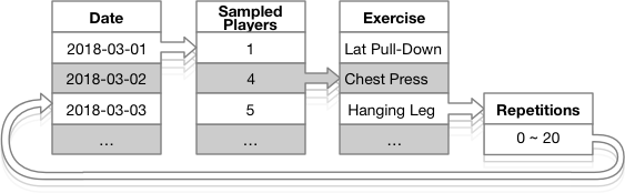
Simulation Process Cycle
Between 15 and 22 players train daily, represented by the Sampled Players in the above graph. Days during the two months where no exercises are simulated are coded those as Day Off.
Some of the exercises repetitions, represented by Repetitions in the graph have a zero count, the case where a player skips an exercise during a training session.
Let’s start this section by creating some parameters and reference values.
Simulation Parameters
# Players: group size
param_group_size <- df %>% nrow()

# Training: Gym exercises + Day off
param_exercises <-
  c(
  "Horizontal Seated Leg Press",
  "Lat Pull-Down",
  "Cable Biceps Bar",
  "Cable Triceps Bar",
  "Chest Press",
  "Hanging Leg Raise",
  "Day Off"
)

# Factor version of the exercises which helps to retain order when graphing
param_exercises_factored <-
  param_exercises %>%
  factor(ordered = TRUE)

# Starting date of the log
param_date_start <- ymd("2018-03-01")

# Creating data ranges, one for 2017 and another for 2018, packaging it nicely
# into a tibble
param_days <-

  tibble(
    Date = c(
      # 2018 data
      seq.Date(
        from = param_date_start,
        by = "day",
        length.out = 28
      ),

      # 2017 data
      seq.Date(
        from = param_date_start - years(1),
        by = "day",
        length.out = 28
      )
    )
  )
Simulation Function
The following code section is the simulation function that maps together the parameters with random combinations and sequences through the simulation process, as represented by the Simulation Process Cycle graph shown above.
func_create_data <-

  # As with the process graph, each day from the param_days tibble is used as a
  # input to start a new simulated cycle
  function(param_day) {

    # Use the integer value of the day to set a seed value, which means that
    # this part of the simulation can be recreated as is
    set.seed(param_day %>% as.integer())

    # create the sample size from the 22 players, sampling a value between 15
    # and 22 which represent the total number of players that exercise in a
    # single day
    training_group_size <- sample(15:param_group_size, 1)

    # Generate between training_group_size-value samples, instanced from a population
    # between 1 to 22 without replacement
    sample(x = 1:param_group_size,
             replace = FALSE,
             size = training_group_size) %>%

      # Map each sampled player in the distribution to all 6 exercises
      purrr::map(function(param_player_number) {
       param_exercises[1:6] %>%

          # for each one of the exercises, create a random sample between 0 and
          # 20 repetitions
          purrr::map(function(param_excercise) {

              # Populate a tibble with all parameters used within the daily
              # cycle simulation.  This part is truly random and will be
              # different between all iterations
            tibble(
              No = param_player_number,
              Exercise = param_excercise,
              Volume = sample(x = 0:20,
                             replace = FALSE,
                             size = 1)
            ) %>%
              return()
          })
      }) %>%

      # Return and nest the result in the daily tibble, corresponding its
      # calling date
      return()
  }
Executing the Simulation
The code section below calls the tmp_exercise_data function by feeding it the previously created parameters.
tmp_exercise_data <-
  param_days %>%

  # Map the list of days to the func_create_data function to simulate the data
  mutate_at(vars(Date), list(data = purrr::map), func_create_data) %>%

  # The unnest() function returns all iteratively nested cycled data to a top
  # param_days level
  unnest(data) %>%
  unnest(data) %>%
  unnest(data) %>%

  # Complete the data for all combinations of the player no, date and exercise,
  # creating explicit entries for the missing combinations
  complete(No, Date, Exercise) %>%

  # Create a new variable by extracting the year value from the date
  mutate_at(vars(Date), list(Year = year)) %>%

  # Group by Player Number and nest the simulated data in the `training_data`
  # column
  group_by(No) %>%
  nest() %>%
  rename(training_data = data)
Explore the Simulated Data
Let’s take a look at the first few rows of player data joined with the simulated data.
df %>%
  select(Player, No) %>%

  # Select the first three players in the list
  head(3) %>%

  # Join the player information (DOB) with the latest year (2018) from the
  # simulated exercise log
  inner_join(tmp_exercise_data %>%
               unnest(training_data) %>%
               filter(Year == max(Year)) %>% # 2018 in this example
               filter(! is.na(Volume)) %>%
               select(-Year)
               ,
             by = "No") %>%
  select(-No) %>%

  # Spread the exercises as columns and populate Volume as its value
  pivot_wider(names_from = Exercise, values_from = Volume) %>%
  group_by(Player) %>%

  # select the top three dates for each of the first three players
  top_n(3, wt = Date) %>%
  kable() %>%
  kable_styling(full_width = FALSE,
                font_size = 9) %>%
  column_spec(1, bold = TRUE) %>%
collapse_rows(columns = 1:1, valign = "top")| Player | Date | Cable Biceps Bar | Cable Triceps Bar | Chest Press | Hanging Leg Raise | Horizontal Seated Leg Press | Lat Pull-Down |
|---|---|---|---|---|---|---|---|
| Jordan Pickford | 2018-03-25 | 11 | 9 | 15 | 16 | 17 | 19 |
| 2018-03-26 | 0 | 0 | 20 | 9 | 16 | 9 | |
| 2018-03-28 | 18 | 13 | 11 | 10 | 15 | 3 | |
| Trent Alexander-Arnold | 2018-03-26 | 1 | 1 | 14 | 13 | 20 | 16 |
| 2018-03-27 | 16 | 3 | 4 | 20 | 9 | 6 | |
| 2018-03-28 | 4 | 10 | 1 | 5 | 18 | 11 | |
| Danny Rose | 2018-03-26 | 7 | 13 | 6 | 5 | 5 | 1 |
| 2018-03-27 | 12 | 12 | 7 | 10 | 10 | 0 | |
| 2018-03-28 | 16 | 13 | 10 | 17 | 19 | 4 |
The following graph shows the cumulative repetitions by player and exercise over a timeline, highlighting the missed training sessions in red.
The func_visualise_day_off function is used to impute a value for the days without exercise data for a player, making it explicit when visualising the data.
func_visualise_day_off <-

  # This function is to explicitly visualise the `Day Off` when graphing the exercise
  # log
  function(df) {
    df %>%

      # Remove all entries with zero volume
      filter(! is.na(Volume)) %>%

      # Extract the entries where all exercises for each player and day
      # combination have zero volume, and overwrite it with 100 in order to
      # visualise it in the context of the exercises
      union_all(
        df %>%
          group_by(No, Date) %>%
          filter(any(is.na(Volume))) %>%
          distinct(No, Date) %>%
          mutate(Exercise = "Day Off",
                 Volume = 100)
      ) %>%
      return()
  }

param_colour_ramp <-

  # Create a colour ramp that maps the colours with the factored exercises, which
  # includes the `Day Off`
  function() {
    # Create an array of colour data
    tmp <- c(viridis::cividis(n = 6), "red")

    # Reorder colour values to align with the exercises and `Day Off`
    tmp <-
      c(
        tmp[1:3], # First 3 exercise colour values
        tmp[7], # Day Off colour in red
        tmp[4:6] # Last 3 exercise colour values
      )
  }

# Create a plot dataframe as we will use filtered parts of it in different geoms
# in the plot
plot_data <-
  df %>%

  # Plot data for the first 9 players in the list
  head(9) %>%

  # Join the exercise log with the player data
  inner_join(
    tmp_exercise_data %>%
      unnest(training_data) %>%
      filter(Year == 2018) %>%

      # Explicitly add in the missing days per player and add volume to plot it
      func_visualise_day_off(),
    by = "No") %>%

  # Convert the exercises into levelled factors to retain the order of the exercises when plotting
  mutate_at(vars(Exercise), factor, levels = param_exercises_factored, ordered = TRUE)

# Now plot the data
plot_data %>%

  # Remove the `Day Off` from the tibble and plot the volume of exercises over
  # the timeline, splitting exercises by colour
  filter(! grepl("day", Exercise, ignore.case = TRUE)) %>%
  ggplot(aes(x = Date, y = Volume, fill = Exercise)) +
  geom_area() +

  # Plot the `Day Off` as bars in the timeline
  geom_col(data  =
             plot_data %>%
             filter(grepl("day", Exercise, ignore.case = TRUE)),
           width = 0.5
           ) +

  # Wrap the plot by player
  facet_wrap(~ Player) +

  # Tidy up the x (data) scale to a suitable format
  scale_x_date(date_labels = "%d-%b") +
  theme_classic() +

  # Manually populate the colour fill values with the function created
  scale_fill_manual(values = param_colour_ramp()) +
  theme(axis.text.x = element_text(angle = 90),
        legend.position = "bottom") +
  labs(title = "English football team training log",
       subtitle = "Volume of reps per exercise & days off over 28 days",
       x = "Date [2018]")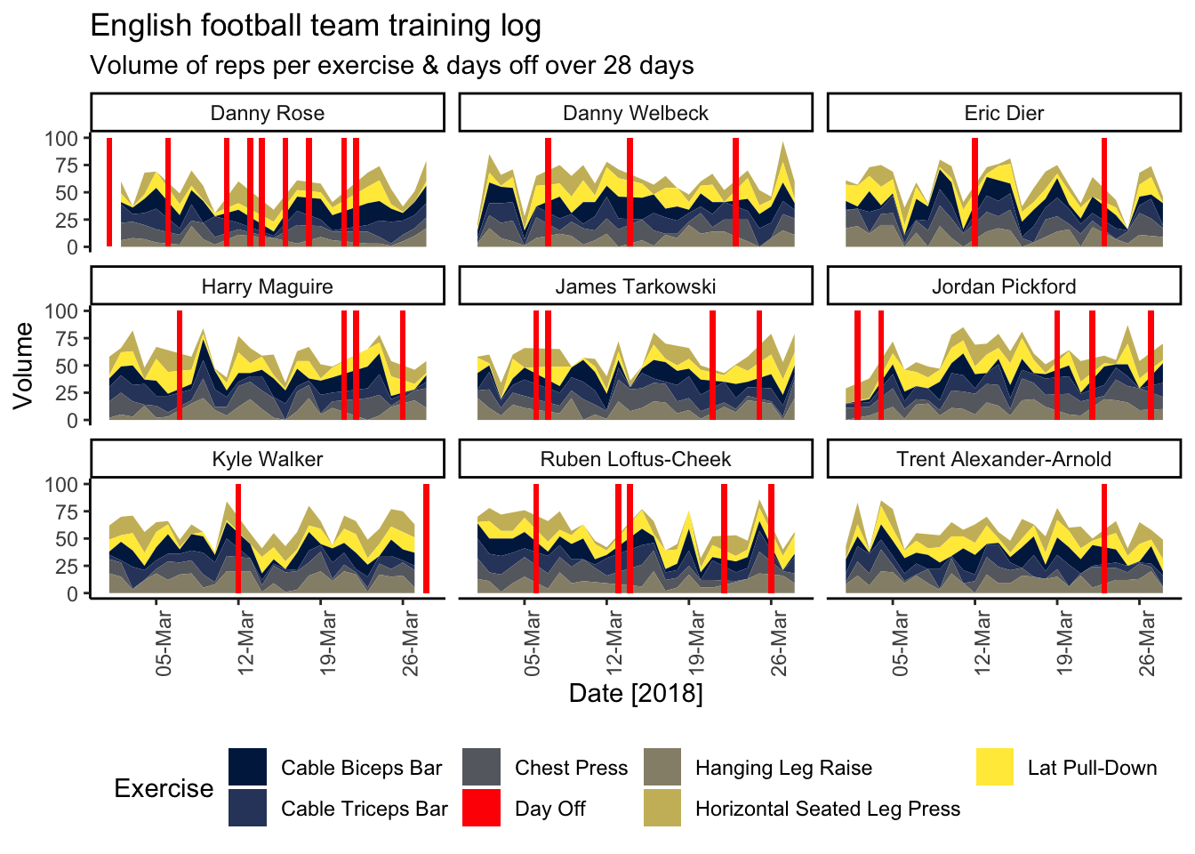
Part 3: Export Simulated Data
Export Process
The aim of this part is to output data into a variety of files to be consumed in Part 4, which is to Import Simulated Data.
The following image shows the process by which data is transformed, grouped and outputted into a variety of file types.
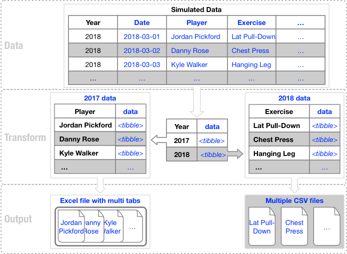
Data Export Process
The training log data is grouped by year, data nested and exported to two file-types, including Excel and CSV.
2017 data is exported to Excel, mapping each player and associated data to a tab. The 2018 data is exported to CSV file-type, with each exercise written to its own file.
To Excel
I use the openxlsx library to create and manipulate Excel files. The aim is to create one Excel file for the 2017 data, creating tabs for each of the 22 players, and populating each sheet with relevant data.
library(openxlsx)

wb <- createWorkbook()
# create workbook instance to populate with tabs and tables

# Join player and simulated data
df_exercise_tab <-
  df %>%
  inner_join(tmp_exercise_data %>%
               unnest(),
             by = "No") %>%

  # Filter on the initial year (2017)
  filter_at("Year", all_vars(. == min(.))) %>%

  # Create new duplicage variable `tab` from Player, using it to group data and
  # output as tabs within the spreadsheet
  mutate(tab = Player) %>%
  group_by(tab) %>%

  # And nest all data for each Player
  nest()

# populate the tabs by walking through the combination of tabs and associated
# data
list(
  df_exercise_tab$tab,
  df_exercise_tab$data
) %>%
  pwalk(function(file_tab, file_data) {

    # add a tab
    addWorksheet(wb, sheetName = file_tab, gridLines = FALSE)
    setColWidths(wb, file_tab, cols = 2:20, widths = 12)

    # Insert a datatable
    writeDataTable(
      wb,
      sheet = file_tab,
      file_data %>% unnest(),
      startCol = "A",
      startRow = 1,
      bandedRows = TRUE,
      tableStyle = "TableStyleLight1"
    )
  })

# IO: Out: Excel
saveWorkbook(
  wb = wb,
  file = paste0(directory_path,
                "england_football_exercise_training_log_2017.xlsx"),
  overwrite = TRUE)
To CSV
Using 2018 data, group data by Exercise and output each to an appropriately named CSV file.
# Join Player data and simulated exercise data
df_exercise_tab <-
  df %>%
  inner_join(tmp_exercise_data %>%
               unnest(cols = c(training_data)),
             by = "No") %>%

  # Filter to retain the max year only (2018)
  filter_at(vars(Year), all_vars(. == max(.))) %>%

  # Create a duplicate variable for Exercise and group by it
  mutate(Exercise_csv = Exercise) %>%
  group_by(Exercise_csv) %>%

  # Nest the data within each exercise
  nest()

# IO: Out: csv
list(
  df_exercise_tab$Exercise_csv,
  df_exercise_tab$data
) %>%

  # Step through list of exercises and nested data
  pwalk(function(csv_name, csv_data) {
    csv_data %>%

      # Write each exercise nested data to a file, appending `2018` to each
      # tidied exercise name to create a file name
      write_csv(
        path = paste0(
          directory_path,  # Directory Path
          csv_name %>%  # Tidied name of the Exercise
            func_rename_tidy() %>%
            str_to_lower(),
          "_2018.csv"  # Add the Year extention
        )
      )
  })
Confirm that the files are created by checking the directory_path folder, as specified in the General Parameters section.
Part 4: Import Simulated Data
Import Process
The aim is to dynamically import data into a common dataframe. With Excel files, the function lists and unnest all the tabs, and import each table back into the calling files tibble as is the case with CSV files.
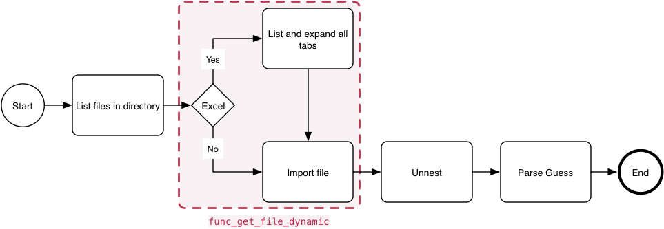
Data Import Process
Import Function
The func_get_file_dynamic function dynamically imports data depending on file-type, depicted in the process graph above.
func_get_file_dynamic <-
  function(file_name) {

    # Check if file name contains .xlsx and map all tabs within it
    if(grepl("xlsx", file_name, ignore.case = TRUE)) {
      tibble(
        file_path = paste(directory_path, file_name, sep = "/"),
        file_tab = excel_sheets(path = paste(directory_path, file_name, sep = "/"))
      ) %>%

        # unnest the list of tabs for each file and import columns with detault
        # `text` datatype
        unnest(file_tab) %>%
        mutate(file = purrr::map2(file_path, file_tab, function(file_path, file_tab) {
          read_excel(path = file_path,
                     col_types = "text",
                     sheet = file_tab,
                     guess_max = 100000)
        })) %>%
        unnest(file) %>%
        return()
    } else {

      # assume that alternative file type is .csv
      read_csv(
        file = paste(directory_path, file_name, sep = "/"),
        guess_max = 100000,

        # set default datatype as text, similar to Excel config
        col_types = cols(.default = col_character())
      ) %>%
        return()
    }
  }
List and import the files
In this section we generate a list of the files located in the directory_path parameter folder, import it using the func_get_file_dynamic function, unnest it and parse_guess the data-types.
files_expanded <-

  # find all files within directory and underlying folders
  list.files(path = directory_path,
           recursive = TRUE) %>%

  # create a tibble of the files and rename the file name to fil_name
  enframe(name = NULL) %>%
  rename(file_name = value) %>%

  # exclude the football file from the results
  filter(! grepl(file_name, pattern = "football\\.csv$", ignore.case = TRUE)) %>%

  # extract the file type for future processing
  mutate_at(vars(file_name), list(file_source = str_extract), pattern = "\\.(csv|xlsx)$") %>%

  # dynamically import the files and nest the file column
  mutate_at(vars(file_name), list(file = purrr::map), func_get_file_dynamic) %>%

  # Unnest all files and consolidate columns, then only guess the data type.
  # This prevents any errors if there are columns with the same file-names but
  # have different datatypes.
  unnest(file) %>%
  mutate_all(parse_guess)
Let’s check the first few rows of the imported data.
# Inspect the first 6 rows of the newly imported files
files_expanded %>%
  head() %>%
  kable() %>%
  kable_styling(full_width = FALSE,
                font_size = 9) %>%
column_spec(1, bold = TRUE)| file_name | file_source | No | Player | DOB | Age | Date | Exercise | Volume | Year | file_path | file_tab |
|---|---|---|---|---|---|---|---|---|---|---|---|
| cable_biceps_bar_2018.csv | .csv | 1 | Jordan Pickford | 1994-03-07 | 25 | 2018-03-01 | Cable Biceps Bar | 0 | 2018 | NA | NA |
| cable_biceps_bar_2018.csv | .csv | 1 | Jordan Pickford | 1994-03-07 | 25 | 2018-03-02 | Cable Biceps Bar | NA | 2018 | NA | NA |
| cable_biceps_bar_2018.csv | .csv | 1 | Jordan Pickford | 1994-03-07 | 25 | 2018-03-03 | Cable Biceps Bar | 3 | 2018 | NA | NA |
| cable_biceps_bar_2018.csv | .csv | 1 | Jordan Pickford | 1994-03-07 | 25 | 2018-03-04 | Cable Biceps Bar | NA | 2018 | NA | NA |
| cable_biceps_bar_2018.csv | .csv | 1 | Jordan Pickford | 1994-03-07 | 25 | 2018-03-05 | Cable Biceps Bar | 9 | 2018 | NA | NA |
| cable_biceps_bar_2018.csv | .csv | 1 | Jordan Pickford | 1994-03-07 | 25 | 2018-03-06 | Cable Biceps Bar | 9 | 2018 | NA | NA |
Visualise Imported Data
Now create a couple of visualisations. The first is the number of records per CSV file or per Excel tab after removing entries with missing or zero volume.
# Visualise the imported file data
files_expanded %>%

  # filter to retain exercises with volume > 0 only, including removing those
  # with NA
  filter(Volume > 0) %>%
  mutate_at(vars(file_tab), ~coalesce(., "None")) %>%

  # This creates a count of rows for combination of file_name, file_tab and
  # file_source
  count(file_name, file_tab, file_source) %>%

  # Create new feature showing tab and file names where relevant:
  # With CSV files:  remove .csv and 2018 from the file name
  # With Excel file: show the tabs only
  mutate(file_tab = case_when(
    grepl(file_name, pattern = "csv", ignore.case = TRUE) ~
      file_name %>%
      str_remove("\\.csv") %>%
      str_remove("\\_2018"),
    TRUE ~ file_tab
  )) %>%

  # Replace the underscore from the file_tab feature with spaces
  mutate_if(is.character, str_replace_all, pattern = "_", replacement = " ") %>%

  # Turn file_tab into factor and order the descending count (n)
  arrange(desc(n)) %>%
  mutate_at(vars(file_tab), fct_inorder) %>%
  ggplot(aes(x = file_tab, y = n, fill = file_source)) +
  geom_col() +
  theme_classic() +
  theme(axis.text.x = element_text(angle = 90, hjust = 1)) +
  scale_fill_viridis_d(option = "E") +
  labs(title = "Number of records by file source",
       subtitle = "Empty records and zero counts removed",
       fill = "File Source",
       x = "File or Tab",
       y = "# Records")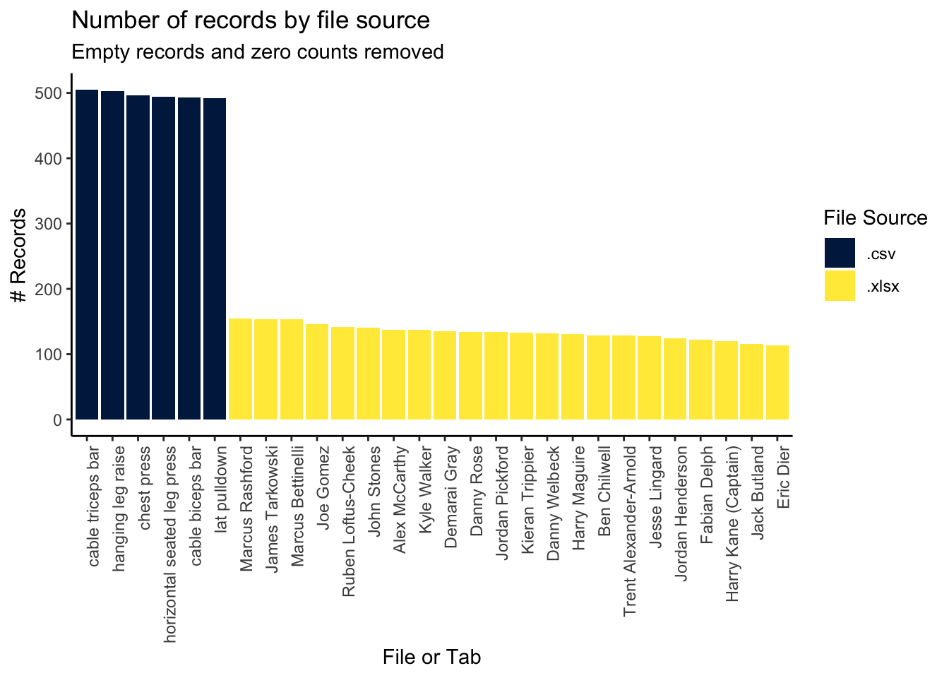
Now combine the file data and create a plot grouped by Player, file type and Year.
# Calculate the average count of records by player
param_player_file_source_ave <-
  files_expanded %>%
  filter(Volume > 0) %>%
  count(Player, file_source) %>%
  ungroup() %>%
  summarise_if(is.numeric, mean) %>%
  pull()

files_expanded %>%
  filter(Volume > 0) %>%
  mutate_at(vars(file_tab), ~coalesce(., "None")) %>%
  count(Player, Year, file_source) %>%
  mutate_if(is.character, str_replace_all, pattern = "_", replacement = " ") %>%
  group_by(Player) %>%
  mutate(total_score = sum(n)) %>%
  arrange(desc(total_score)) %>%
  ungroup() %>%
  mutate_at(vars(Player), fct_inorder) %>%
  ggplot(aes(x = Player, y = n, fill = n)) +
  geom_col() +
  geom_hline(yintercept = param_player_file_source_ave,
             col = "red",
             lty = 2,
             size = 0.5
             ) +
  annotate("text",
           x = 5,
           y = param_player_file_source_ave + 20,
           label = paste("Average:", round(param_player_file_source_ave)),
           col = "red",
           size = 4
           ) +
  facet_grid(file_source + Year ~ .) +
  scale_fill_viridis_c() +
  theme_classic() +
  theme(axis.text.x = element_text(angle = 90, hjust = 1)) +
  labs(title = "Number of records by player and file source",
       subtitle = "Empty records and zero counts removed",
       fill = "# Records",
       x = "Player",
       y = "# Records")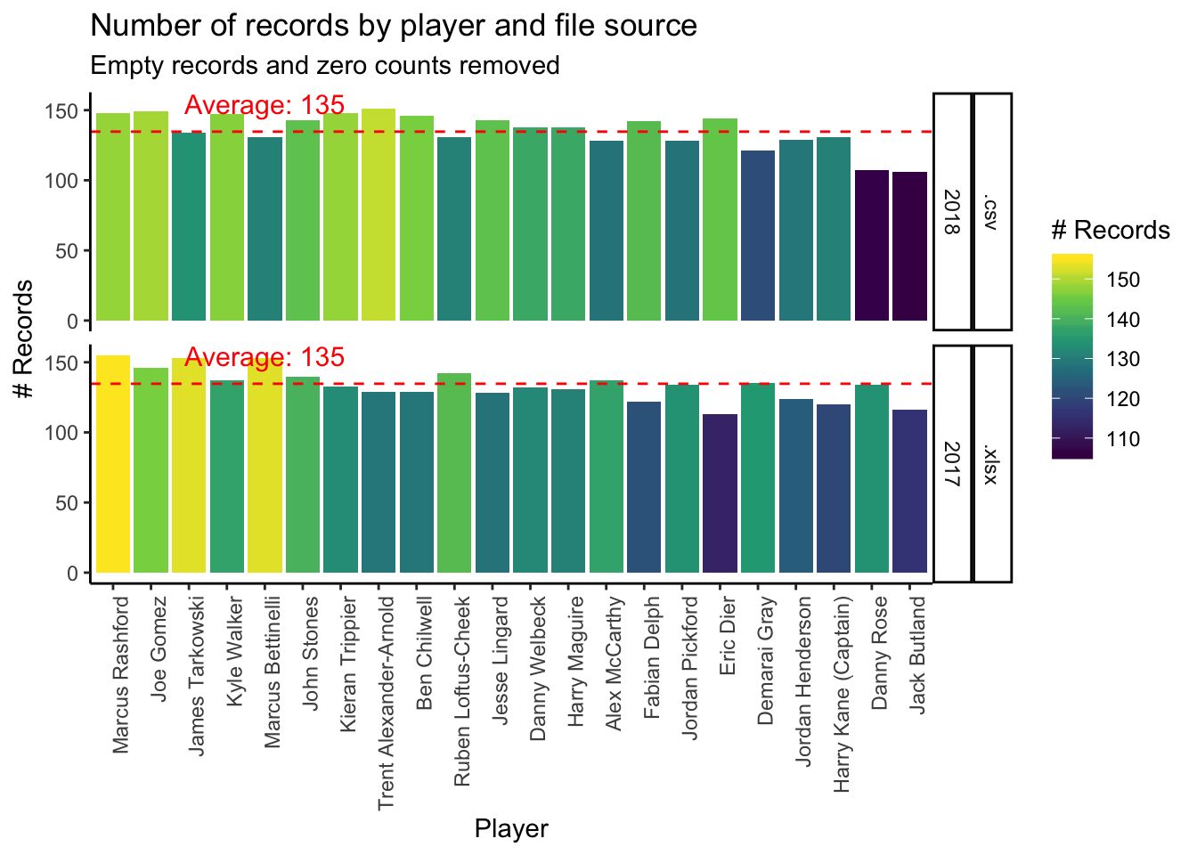
Summary
This tutorial is simplified and without real-world nuances and overhead, like error handling for example. However, the power and simplicity of the approach is adequately demonstrated and can be extended for use in similar situations.
Session Info
## R version 3.6.2 (2019-12-12)
## Platform: x86_64-apple-darwin15.6.0 (64-bit)
## Running under: macOS Catalina 10.15.3
##
## Matrix products: default
## BLAS:   /Library/Frameworks/R.framework/Versions/3.6/Resources/lib/libRblas.0.dylib
## LAPACK: /Library/Frameworks/R.framework/Versions/3.6/Resources/lib/libRlapack.dylib
##
## locale:
## [1] en_GB.UTF-8/en_GB.UTF-8/en_GB.UTF-8/C/en_GB.UTF-8/en_GB.UTF-8
##
## attached base packages:
## [1] stats     graphics  grDevices utils     datasets  methods   base
##
## other attached packages:
##  [1] openxlsx_4.1.4   kableExtra_1.1.0 knitr_1.28       readxl_1.3.1
##  [5] lubridate_1.7.4  forcats_0.4.0    stringr_1.4.0    dplyr_0.8.4
##  [9] purrr_0.3.3      readr_1.3.1      tidyr_1.0.2      tibble_2.1.3
## [13] ggplot2_3.2.1    tidyverse_1.3.0
##
## loaded via a namespace (and not attached):
##  [1] Rcpp_1.0.3        lattice_0.20-40   assertthat_0.2.1  digest_0.6.24
##  [5] plyr_1.8.5        R6_2.4.1          cellranger_1.1.0  backports_1.1.5
##  [9] reprex_0.3.0      evaluate_0.14     httr_1.4.1        highr_0.8
## [13] blogdown_0.17     pillar_1.4.3      rlang_0.4.4       lazyeval_0.2.2
## [17] rstudioapi_0.11   rmarkdown_2.1     labeling_0.3      webshot_0.5.2
## [21] selectr_0.4-2     munsell_0.5.0     broom_0.5.4       compiler_3.6.2
## [25] modelr_0.1.5      xfun_0.12         pkgconfig_2.0.3   htmltools_0.4.0
## [29] tidyselect_1.0.0  gridExtra_2.3     bookdown_0.17     fansi_0.4.1
## [33] viridisLite_0.3.0 crayon_1.3.4      dbplyr_1.4.2      withr_2.1.2
## [37] grid_3.6.2        nlme_3.1-144      jsonlite_1.6.1    gtable_0.3.0
## [41] lifecycle_0.1.0   DBI_1.1.0         magrittr_1.5      scales_1.1.0
## [45] zip_2.0.4         cli_2.0.1         stringi_1.4.6     reshape2_1.4.3
## [49] farver_2.0.3      viridis_0.5.1     fs_1.3.1          xml2_1.2.2
## [53] ellipsis_0.3.0    generics_0.0.2    vctrs_0.2.3       tools_3.6.2
## [57] glue_1.3.1        hms_0.5.3         yaml_2.2.1        colorspace_1.4-1
## [61] rvest_0.3.5       haven_2.2.0
IO: in/ out or input and output for data↩︎